Four source mechanisms matter most.

First, there is particle wall friction. This is present during ordinary flow. Particles slide, catch, release, and transmit energy into the wall. In many powder systems, this is the baseline signal. It changes with wall condition, surface films, particle shape, velocity, and stress state.

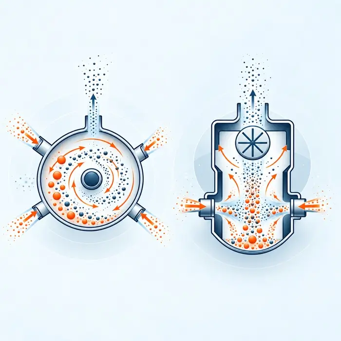
Second, there are particle impacts. In more dilute conveying or in high-energy transition zones, these impacts can dominate. Bends, transitions, and feed points are especially active. Acoustic methods have been used to estimate mass flow rate and even aspects of particle size under these conditions, although the signal processing burden rises fast as the flow becomes more complex.

Third, there is particle breakage or damage. This matters in friable systems, in feeders, during granulation, and in processes where morphology changes with handling. It is useful, but it is a different problem from blockage prediction.

Fourth, there is a changing contact structure under consolidation. This is the part that matters most for blockage warning. As a powder moves from stable flow toward unstable discharge, the contact network changes. Stress localizes. Slip becomes intermittent. Temporary structures form and release. In practical terms, the signal often shifts from a more continuous background toward a more uneven burst pattern or toward a persistent loss of the previous activity level, depending on the process and the measurement point. That is the useful moment. A good system detects the transition in flow state before the plant reaches a full stop.

Blockages rarely appear out of nowhere. The sequence is usually progressive.

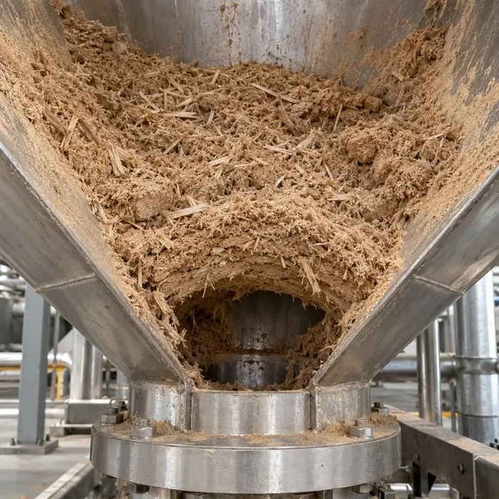
The flow starts steadily. Then something changes. A fine-rich lot enters the line. Humidity drifts. A wall film develops. Attrition broadens the PSD during transfer. A local section deaerates differently. Velocity drops in one region. Stresses rise above it. Discharge becomes less uniform. In a hopper, that can mean intermittent support structures, partial collapse, then a stable arch or a rathole. In a conveying line, it can mean changing solids concentration, unstable slugging behavior, or localized deposition that keeps building.

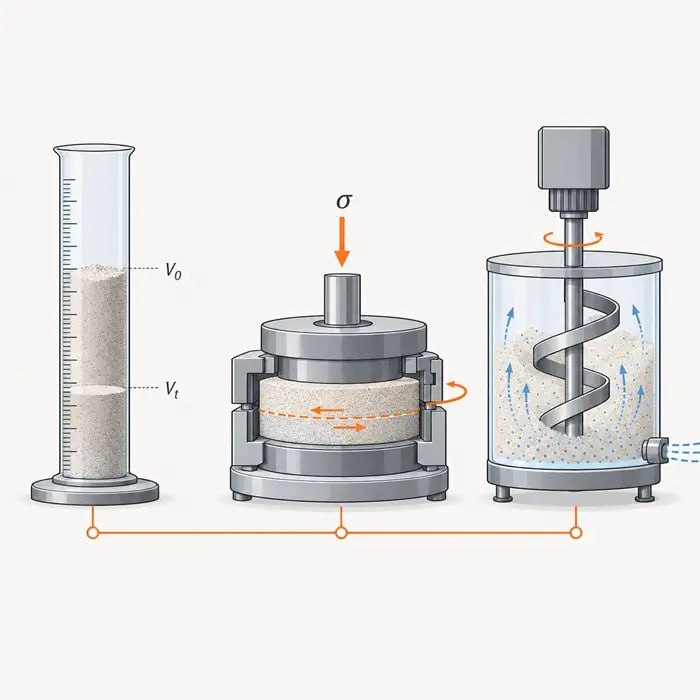
That is why acoustic emission is best understood as a regime change detector first. It can become a blockage predictor when the deterioration pattern is repeatable and the sensors are placed close enough to the failure zone. This is also why you should not treat it as a substitute for basic solids engineering. If a bin is already vulnerable to arching, powder flowability, wall friction, and hopper geometry, the correct powder flow test method still decides whether the vessel will discharge cleanly. Acoustic emission helps you detect the shift. It does not repeal powder mechanics.

Raw acoustic data is useless in a plant. It is too rich, too noisy, and too sensitive to everything around it.

The first step is filtering. Most systems try to separate process-related activity from ordinary mechanical vibration and electrical contamination. That sounds easy. It is not. A clean band in one plant can be polluted in another by structure-borne vibration, loose mounts, bearing defects, or resonance in the frame.

The second step is feature extraction. This is where the method becomes practical. Instead of feeding entire waveforms into the control layer, the system turns short windows of data into manageable features such as RMS, energy distribution, count-based measures, frequency descriptors, or wavelet-based features. That approach is visible across the literature, from pneumatic conveying and screw feeders to mixing and granulation.

The third step is classification or prediction. This is where people often get overconfident. Machine learning can improve performance. It can reduce error and classify regimes better than blunt thresholds alone. However, the same literature also shows the real limitation. Models trained in one setup do not transfer cleanly to another unless the training strategy accounts for flow regime, geometry, material, and signal standardization. In plain English, lab data does not magically become plant data. If the model has never seen your powder, your pipe, your feeder, or your noise environment, the output should be treated with suspicion.

Read the MDPI’s article – Detection of Pneumatic Conveying by Acoustic Emissions

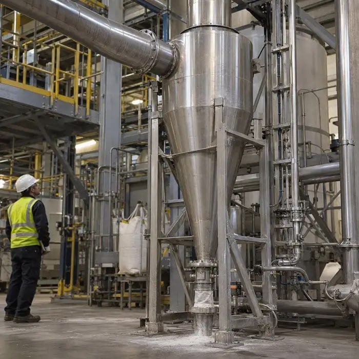
Sensor placement sounds straightforward until you try to do it properly. For hoppers, the useful zone is often around the lower cone, the outlet, or the region where intermittent support structures are expected to form. For conveying systems, bends, transitions, and sections known for deposition or unstable flow are better candidates than long, quiet straight runs. For feeders, the mounting point has to reflect where the structure picks up process-related activity rather than general drive noise.

Mounting quality matters. Coupling matters. Surface condition matters. Acoustic emission is a structure-borne measurement. A sloppy mount, a painted contact area, or a poor mechanical path can weaken the very signal you care about. Just as important, attenuation is real. These sensors are local instruments. They are strong when they sit near the physics that matters. They are weak when you expect one sensor to explain a whole line.

The output path matters too. An alarm that fires when the flow has already stopped is of limited value. The real benefit comes when the signal is tied to action. That may mean slowing feed, changing aeration, triggering a controlled intervention, or pushing a warning to the DCS early enough for an operator to respond.

Most first installations tend to fail for boring reasons. They fail because the project expects one universal threshold. They fail because the sensor sits where installation is easy, not where the failure starts. They fail because the team trains on ideal material, then runs production with humidity drift, fines growth, recycled material, or changing wall conditions. They fail because the algorithm was tuned during commissioning and never updated after the plant changed. They fail because the system is sold as a blockage prediction when it is actually only a flow condition monitor.

There is another trap. Acoustic emission often picks up real changes that are not blockage precursors. That is not a flaw in the sensor. It is a flaw in the interpretation. A conveying line may sound different because pneumatic conveying attrition has changed the powder. A hopper may sound different because moisture control for powders has drifted outside the useful window. A blend may destabilize because segregation in blending and transport is changing what arrives at the discharge point. In that sense, acoustic emission can be valuable even when it does not predict a plug directly. It can tell you that the material state has changed before the plant gives you a visible failure.

Used well, acoustic emission fits in three places. It works as a local early warning layer on assets with repeatable failure zones, as well as a process condition monitor where flow regime changes matter even before a true blockage. Additionally, it works as part of a hybrid strategy, alongside solids testing, pressure data, throughput trends, and practical knowledge of the line.

That third use is usually the strongest. If a hopper repeatedly shows symptoms that point to consolidation-driven failure, start with the mechanics. Check if the outlet is undersized. Check the wall friction. Check the moisture window. Confirm the relevant stress state with the right test. Then use acoustic emission to monitor drift away from the known good operating state. That is a serious engineering workflow. It is far better than pretending a sensor can rescue a weak design.

Acoustic emission for flow blockage prediction is real. It is useful. It is also easy to oversell.

The method is strongest when the failure zone is known, the signal path is short, the background noise is understood, and the model has been built around the real plant. Under those conditions, acoustic emission can detect degrading flow early enough to matter. Outside those conditions, it often remains useful as a regime change monitor, but not as a universal predictor of every future plug.

That is the practical answer. The method works. The installation decides whether it works for you.