
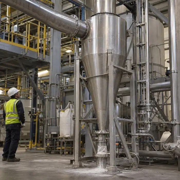
A cyclone that previously separated powder reliably begins sending more fines to the coarse outlet. The feed particle size distribution (PSD) appears unchanged, the fan is running normally, and the calculated cut size still meets the specification. Increasing inlet velocity seems like an obvious correction. But what if the cyclone is no longer separating the individual particles shown in the laboratory report?
Cohesive fines can enter as agglomerates, adhere to larger particles, or accumulate on cyclone walls. A leaking dust discharge can disturb the vortex and return collected material to the gas stream. These problems may produce similar changes in the outlet PSD, yet they call for entirely different solutions. The challenge is to establish what changed before adjusting the equipment.
How a Cyclone Separates Particles
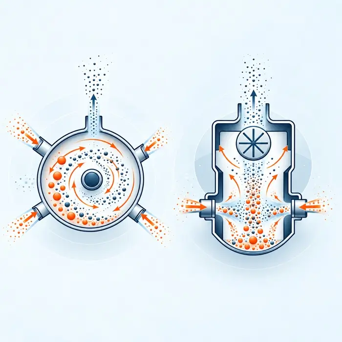
In a reverse-flow gas cyclone, particle-laden gas enters tangentially and establishes a swirling flow. Larger or denser particles generally migrate toward the outer wall, while smaller particles follow the inward-moving gas toward the vortex finder. Separation depends on particle inertia, gas drag, turbulent dispersion, residence time, and the velocity field within the cyclone.
Particles reaching the collection region move toward the lower dust discharge. The cleaned gas reverses direction, forming an inner vortex that leaves through the upper outlet.
The distinction between collected and escaping particles is not absolute. A cyclone collects some particles below its nominal cut size and loses some larger ones. The cut size, d50, identifies the particle diameter collected at 50% grade efficiency under specified operating conditions.
Estimating Cut Size with the Lapple Model
The Lapple relationship provides a first estimate of cut size:
The calculation uses gas viscosity (μ), cyclone inlet width (b), effective gas turns (Ne), inlet velocity (Vi), and the difference between particle and gas density (ρp − ρg). With SI units, the result is expressed in meters. The equation assumes a simplified particle migration mechanism governed by Stokes drag. It is useful for initial design comparisons within an appropriate cyclone geometry, but it does not represent the complete internal flow.
The effective number of gas turns can be estimated from the cyclone dimensions:
Here, Lb is the cylindrical body height, Lc is the cone height, and H is the inlet height.
For a cyclone with a cylindrical height of 0.30 m, cone height of 0.40 m, and inlet height of 0.10 m:
This gives the five effective turns used in the following calculation. The value is a geometric estimate rather than a measurement of the gas’s actual path through the cyclone.
Another useful measure is the Stokes number:
In this expression, dp is particle diameter, U is a characteristic gas velocity, and L is a characteristic dimension of the cyclone. The equation assumes spherical particles in the low-Reynolds-number drag regime.
The Stokes number compares particle inertia with the characteristic timescale of the gas flow. It provides a useful basis for comparing separation behavior, although the characteristic dimensions and critical Stokes number depend on the cyclone model.
Worked Calculation: A Nominal 3.7 µm Cut
Consider a cyclone handling particles with a density of 2,500 kg/m³ in air at an inlet velocity of 15 m/s.
| Parameter | Assumed value |
|---|---|
| Gas viscosity, μ | 1.8 × 10⁻⁵ Pa·s |
| Cyclone inlet width, b | 0.10 m |
| Effective gas turns, Ne | 5 |
| Inlet velocity, Vi | 15 m/s |
| Particle density, ρp | 2,500 kg/m³ |
| Gas density, ρg | Approximately 1.2 kg/m³ |
Substituting these values into the Lapple equation gives a nominal cut size of approximately 3.7 µm. That is a useful starting point for evaluating the design, but it is not a sharp separation boundary. Particles larger than 3.7 µm can still escape, and smaller particles can still be collected. The calculation also assumes a particle population whose aerodynamic properties can be represented by the selected density and diameter.
Why More Inlet Velocity Is Not Always Better
The Lapple relationship predicts that cut size decreases with the square root of inlet velocity. Doubling the velocity from 15 to 30 m/s would reduce the calculated cut size from approximately 3.7 to 2.6 µm, an improvement of about 29%. The pressure-drop penalty is considerably larger. For unchanged cyclone geometry and an approximately constant loss coefficient, pressure drop scales with velocity squared. Doubling velocity therefore increases pressure drop by roughly a factor of four.
This is a substantial increase in pressure loss for a comparatively modest reduction in nominal cut size. Higher velocity also changes turbulence, particle-wall impacts, and the risk of re-entrainment. Kalen and Zenz (1974) examined cyclone saltation velocity, a concept that helps explain why collection efficiency can reach a maximum rather than improve indefinitely. Saltation velocity is a model-dependent reference, not a fixed maximum operating speed.
Before increasing velocity, establish whether the existing flow rate is actually responsible for the observed problem.
When Muschelknautz Is More Useful Than Lapple
Lapple’s equation is convenient because it requires relatively few inputs. The same simplicity limits its usefulness when the cyclone’s internal flow and particle loading become important. The Muschelknautz approach treats the gas velocity field, wall friction, and solids loading in greater detail. Its limit-loading concept describes how much particulate material can remain suspended in the rotating gas flow. Beyond that loading condition, particle transport and collection behavior change.
Hoffmann and Stein’s Gas Cyclones and Swirl Tubes (2008) provides a detailed treatment of the theory and its application to industrial cyclone design. Geometry also influences pressure loss. Elsayed and Lacor (2010) combined mathematical modeling and computational fluid dynamics to investigate cyclone dimensions that minimize pressure drop. Their work concerns hydraulic and geometric optimization rather than direct validation of the Muschelknautz limit-loading concept.
For a preliminary equipment comparison, Lapple may be sufficient. For an industrial design where pressure loss, internal flow, and particle loading materially affect the outcome, a more detailed model is justified.
Reading the Grade Efficiency Curve
A cut-size estimate gives only one point on the cyclone’s separation curve. Grade efficiency describes how the collected fraction varies across particle sizes.
Theodore and DePaola (1980) fitted the following fractional-efficiency expression to Lapple’s experimental data:
Here, η(d) is the fraction collected from particles of diameter d, and d50 is the particle size at which collection efficiency reaches 50%.
Using the calculated 3.7 µm cut size gives:
| Particle size | Predicted grade efficiency |
|---|---|
| 2 µm | Approximately 23% |
| 3.7 µm | 50% |
| 8 µm | Approximately 82% |
The figures show why a nominal cut size should never be interpreted as a perfect separation boundary. Even at 8 µm, the simplified model predicts that some material escapes.
Actual efficiency curves depend on the cyclone design and operating conditions. Dirgo and Leith (1985) compared measured cyclone efficiencies with theoretical predictions, demonstrating the importance of testing the assumptions behind a model.
Cut Size Is Not Enough: Curve Sharpness Matters
Two cyclones with the same d50 can produce different product size distributions because the transition between collection and escape is not equally sharp.
One measure of separation sharpness is:
The terms d25 and d75 identify the particle sizes collected at 25% and 75% grade efficiency. With this definition, a value closer to 1 indicates a sharper separation. For the Theodore and DePaola curve, d25 is approximately 0.577 d50 and d75 is approximately 1.732 d50. The resulting sharpness index is about 0.33. Some references use the reciprocal, d75/d25. Comparing reported sharpness values without checking the convention can therefore produce misleading conclusions.
When the process requires a narrow product PSD, curve sharpness and the amount of misplaced material deserve as much attention as the nominal cut size.
Reconstructing Grade Efficiency from Plant Samples
A grade efficiency curve must be calculated from representative stream measurements and a material balance. Comparing normalized feed and outlet PSD curves alone is insufficient.
For particle-size class i:
Here, Mf is the total feed solids mass during the sampling period, Mc is the collected coarse-outlet solids mass, and wf,i and wc,i are the corresponding mass fractions in size class i. For continuous operation, measured mass flow rates can replace total masses, provided they refer to the same steady operating period.
Samples from the feed, coarse discharge, and gas outlet must represent that period. Where particles are carried in the outlet gas, isokinetic sampling may be required to avoid particle-size bias. The dust discharge must also be sampled without breaking its pressure seal.
The fines-outlet solids mass provides a check on the overall material balance. Material retained in ducts, deposits inside the cyclone, and sampling losses must be considered when interpreting the result. Use the same PSD measurement basis for the three streams. Differences in sample dispersion can otherwise appear as differences in collection efficiency.
Why the Fine End Can Behave Differently
Some measured efficiency curves show an increase in collection at the smallest particle sizes, commonly described as the fish-hook effect. One explanation is agglomeration. Paiva, Salcedo, and Araujo (2010) modeled particle collisions and agglomeration in a cyclone and showed how aggregates can follow trajectories different from those of their constituent particles.
Fine particles that enter or form part of larger clusters may therefore be collected more readily than their primary particle sizes would suggest. A similar curve shape can also result from sampling or PSD measurement errors. Before treating a fish-hook pattern as evidence of agglomeration, check the stream balance and the particle size measurement procedure.
Where Cohesive Fines Change the Separation
Most conventional cyclone calculations assume the aerodynamic properties of the entering particle population can be described using particle size, density, and shape. For cohesive fines, those properties may change during handling and separation.
Fine particles attract one another through van der Waals forces, electrostatic interactions, and, under suitable moisture conditions, liquid bridges. They can enter the cyclone as clusters, collide and form new aggregates, or break apart under acceleration and wall impacts. The cyclone responds to the aerodynamic units present in its flow field, not necessarily the primary particles measured after laboratory dispersion.
Agglomerate Size Is Not Aerodynamic Size
A loose agglomerate does not behave like a compact sphere with the same outer diameter. Its porosity, effective density, shape, and drag determine how it moves through the gas. Sgrott Júnior and Sommerfeld (2019) investigated particle collisions and agglomeration in a gas cyclone using coupled fluid-particle simulation. Their work demonstrates the importance of particle interactions and aggregate structure when predicting collection.
Paiva and colleagues (2010) also showed that accounting for agglomeration changes the predicted collection of fine particles compared with treating every particle as an independent unit. This is the central weakness of applying a primary-particle cut-size calculation directly to a cohesive feed. The cyclone may be processing clusters whose aerodynamic behavior differs substantially from the individual particles used in the calculation.
Moisture and Electrostatics Change the Feed Before Entry
Agglomeration often begins upstream. Adsorbed moisture can strengthen particle contacts or form liquid bridges. The resulting cohesion depends on humidity, temperature, surface chemistry, and the powder’s moisture sensitivity. Two lots with similar bulk moisture contents can behave differently when their surface conditions differ.
Inlet-gas humidity, dew point, and powder storage conditions therefore belong in the investigation. PTI’s Moisture Control for Powders explains how these conditions relate to caking and particle cohesion.
Electrostatic charging is another possible contributor. Contact during milling and conveying can charge particles, encouraging fines to adhere to equipment surfaces, larger particles, or one another. See Electrostatic Effects in Powder Handling. Neither mechanism is necessarily evident from a PSD measurement performed after strong dispersion.
Cohesive Fines Can Change the Cyclone Itself
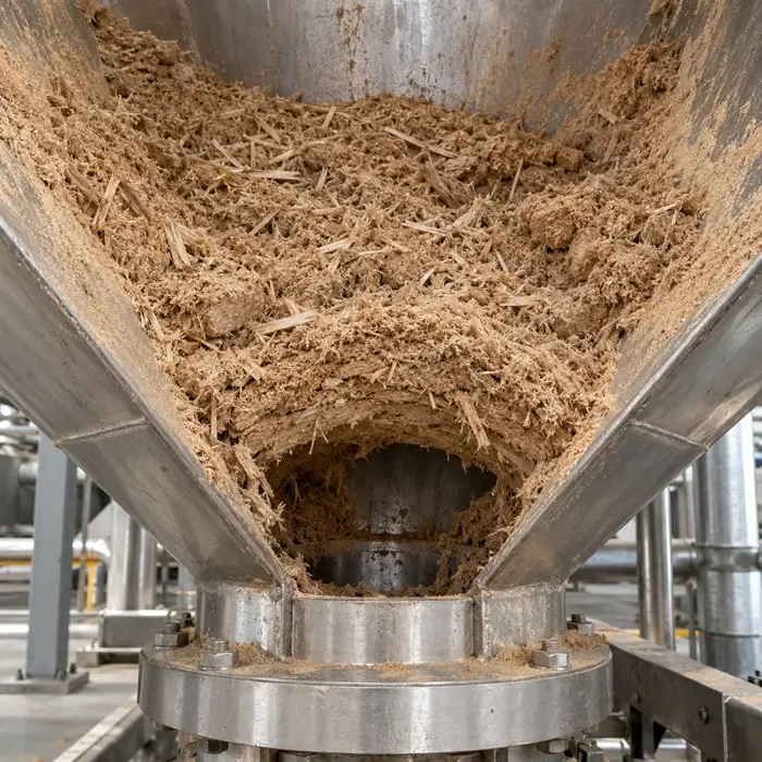
Fine material can accumulate on the cone, barrel wall, and vortex finder. As deposits grow, they change the effective flow passage and wall condition. They can disturb the vortex, promote local re-entrainment, or restrict the lower dust discharge. The problem then involves both the material entering the cyclone and the equipment geometry through which it travels. A change in feed cohesion can produce a change in operating performance even when the cyclone’s original dimensions and gas-flow setpoint remain unchanged.
Before Blaming the Powder, Check the Cyclone
<p>A sudden deterioration in separation should trigger a mechanical and operating check before a detailed investigation of powder agglomeration.</p>
1. Dust Outlet Air Leakage
A worn rotary airlock, leaking discharge connection, damaged seal, or poorly seated flap valve can admit air into a cyclone operating under negative pressure. Air entering through the dust discharge disturbs the lower vortex and can re-entrain particles that have already reached the collection region.
The US EPA’s cyclone monitoring guidance identifies air inleakage, plugging, and erosion as common causes of reduced cyclone performance. Inspect the rotary valve clearances, dust receiver connections, hopper pressure, and seals. Correcting a discharge leak may restore separation without changing the cyclone’s operating point.
2. Wall Deposition and Dust Discharge
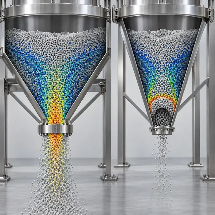
Inspect the cone, barrel wall, and vortex finder for buildup. Check whether the dust hopper is bridging or material is backing up into the collection region. Deposits can change the gas-flow field, while a restricted discharge prevents collected solids from leaving as intended. Both problems should be corrected before interpreting a change in measured grade efficiency as a failure of the cyclone design.
3. Gas Flow and Pressure Drop
Measure the actual inlet flow rate, gas temperature, density, and cyclone pressure drop. Compare the results with the historical operating condition. Fan speed alone is not a sufficient check. Changes in upstream or downstream pressure losses can alter the flow rate through the cyclone even when fan speed remains constant.
4. Solids Loading
Record the solids feed rate and gas volume flow so the inlet mass loading can be compared with previous operating conditions. The effect is not merely hydraulic. Particle concentration influences collisions, turbulence, and agglomeration. The Muschelknautz approach recognizes a limit to the amount of solids that can remain suspended in the rotating gas.
Ji et al. (2009) studied calcium carbonate separation at particle concentrations from 5 to 2,000 mg/m³ and inlet velocities from 6 to 30 m/s. Within the investigated range, increasing concentration and velocity improved overall and grade efficiencies, with agglomeration contributing to the observed behavior. The result is specific to the tested conditions. It establishes solids loading as a variable that must be recorded and controlled when comparing cyclone performance.
Reading PSD Data Without Destroying the Evidence
<p>A laboratory PSD represents the particles and any remaining agglomerates under the dispersion conditions used for measurement. That distinction matters when a cyclone processes cohesive material. Strong dry dispersion can break apart clusters that survived during separation. Two feed samples with different agglomeration states may consequently produce similar PSDs after sufficiently strong dispersion.</p>
Use a Dry Dispersion Pressure Titration
For suitable powders, dry laser diffraction can be used to examine how the measured distribution changes with dispersion pressure. A practical initial investigation might cover approximately 0.5 to 4 bar, depending on the instrument and material. Use representative subsamples at successive pressure settings and record D10, D50, D90, and the relevant size fractions. At low pressure, loosely bound agglomerates may remain intact, producing a coarser apparent distribution. As pressure increases, the clusters disperse and the PSD becomes finer.
The important point is the first stable plateau, where further increases in pressure produce little additional change. Beyond that plateau, renewed fining needs investigation. Excessive dispersion energy may fracture primary particles rather than simply separate agglomerates. Microscopy or another suitable imaging method can help distinguish those mechanisms.
Jaffari et al. (2013) investigated seven pharmaceutical inhalation powders over dry dispersion pressures of 0.2 to 4.5 bar. Their measured critical primary pressures, indicating the onset of complete deagglomeration under the test conditions, ranged from 1.0 to 3.5 bar. Although the materials differed from typical industrial cyclone feeds, the study demonstrates how dispersion-pressure titration can be used to assess powder agglomeration.
ISO 13320:2020 provides the framework for laser diffraction method selection and validation. The dispersion protocol should accompany the reported PSD, particularly when results are used to investigate changes in separation.
Representative sampling is equally important. A properly operated rotary riffler reduces the sampling bias associated with taking an unstructured scoop from a powder container.
Reconstruct the Stream Balance
Collect representative feed and outlet samples over the same stable operating period, measure the corresponding solids flows, and verify that the material balance closes within the required uncertainty. Run the primary PSD measurements using a consistent dispersion procedure. If agglomeration is suspected, repeat selected samples under gentler conditions as a separate investigation. This distinguishes the fraction of each measured size class reporting to each outlet from the question of whether those size classes existed as separate particles inside the cyclone. The first is a mass-balance problem. The second is a question of particle structure and process history.
Worked Troubleshooting Example: More Fines in the Coarse Discharge
Illustrative example, not experimental data:
Suppose the coarse discharge of a cyclone starts showing a higher proportion of particles below 10 µm. Nothing obvious has changed in the feed PSD, at least not when the samples are measured under strong dispersion. The first suspicion might be that the cyclone has lost some of its separation efficiency. But an increase in fines measured in the coarse discharge doesn’t tell us why those particles ended up there.
Start with the cyclone itself. A leaking rotary valve can disturb the lower vortex, deposits can change the effective geometry, and a shift in gas flow or solids loading can alter the separation. Check these against the previous operating conditions before drawing conclusions from the PSD.
Now suppose those checks reveal nothing unusual. The airlock is sealing properly, the cone and vortex finder are clear, and gas flow, pressure drop, and solids loading remain within their normal ranges. That leaves the powder worth examining more closely.
The strongly dispersed PSD looks much like the historical reference, but a second measurement at lower dispersion pressure shows a coarser distribution. Increasing dispersion pressure progressively reduces the apparent particle size until the distribution stabilizes. That is consistent with agglomerates being broken apart during measurement. The storage records also show higher humidity exposure than usual. This doesn’t establish that moisture caused the change, but it gives the investigation a direction.
The useful next test is a comparison of the same powder conditioned at the previous and current humidity levels, with cyclone operating conditions held constant. If the outlet split changes consistently with conditioning, the evidence points toward the feed’s agglomeration state rather than a mechanical problem. At that point, storage humidity control or upstream deagglomeration becomes a more sensible intervention than increasing cyclone velocity. The result should still be confirmed through representative stream sampling and a solids mass balance before changing the operating specification.
When Shear or Cohesion Testing Helps
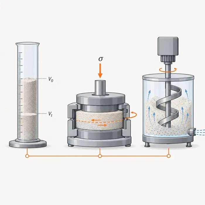
Shear cell testing measures bulk powder strength under controlled consolidation. It can establish whether changes in powder condition have altered cohesion, an important consideration for storage and feeding. It cannot directly measure whether airborne agglomerates will survive acceleration, collisions, and turbulent shear inside a cyclone.
Dynamic and aerated powder testing adds information about powder response under imposed motion and gas flow. The measurements are useful, but their laboratory stress and aeration conditions do not reproduce the complete cyclone flow field. For cohesive fines, use these methods to support PSD dispersion studies, conditioning experiments, and representative separation trials. A rise in bulk cohesion gives engineers a reason to investigate agglomeration, not a direct prediction of cyclone cut size.
What Should the Engineer Change?
Once the cause of the changed separation is identified, the options become more specific.
| Finding | Practical response |
|---|---|
| Dust-outlet air leakage | Repair rotary valve seals and restore discharge integrity |
| Deposits or bridging | Remove buildup, correct restrictions, and investigate moisture and cleaning requirements |
| Humidity-driven agglomeration | Specify storage and inlet-gas humidity or dew point limits based on conditioning tests |
| Agglomerates entering the cyclone | Evaluate controlled upstream deagglomeration without unacceptable particle breakage |
| Changed solids loading | Reassess the operating point and loading-dependent separation behavior |
| Stable but different feed condition | Requalify the process if the revised product split meets requirements |
| Need for a sharper fine-particle split | Consider an air classifier with active dispersion rather than relying on a conventional cyclone |
A conventional gas cyclone is a reliable separator for many applications, but it is not necessarily the right equipment when a cohesive fine powder requires a narrow, sharply controlled product PSD. PTI’s Size Reduction & Classification guide examines the equipment options in relation to target PSD, throughput, powder behavior, and yield. The broader Process & Equipment hub connects these decisions with upstream feeding, conveying, and downstream handling.
The Qualification Question
The real qualification task is to define the conditions under which the cyclone delivers the required product split. For stable, free-flowing powders, a validated cut-size estimate and representative performance measurements may be enough. Cohesive fines require additional control over feed conditioning, agglomeration state, PSD dispersion, inlet-gas conditions, solids loading, and dust-discharge integrity. A cyclone does not separate the particle sizes printed on a laboratory report. It separates the aerodynamic units entering its vortex, under the equipment and operating conditions present at that moment. When separation drifts, determine whether the machine changed, the powder changed, or both.
FAQ: Cyclone Separation of Fine Powders
Technical Basis / Sources
- Hoffmann, A. C., and Stein, L. E. (2008). Gas Cyclones and Swirl Tubes: Principles, Design, and Operation, 2nd edition. Springer.
- Theodore, L., and DePaola, V. (1980). Predicting Cyclone Efficiency. Journal of the Air Pollution Control Association, 30(10), 1132–1133.
- Dirgo, J., and Leith, D. (1985). Cyclone Collection Efficiency: Comparison of Experimental Results with Theoretical Predictions. Aerosol Science and Technology, 4(4), 401–415.
- Kalen, B., and Zenz, F. A. (1974). Theoretical-Empirical Approach to Saltation Velocity in Cyclone Design. AIChE Symposium Series, 70(137), 388–396.
- Elsayed, K., and Lacor, C. (2010). Optimization of the Cyclone Separator Geometry for Minimum Pressure Drop Using Mathematical Models and CFD Simulations. Chemical Engineering Science, 65(22), 6048–6058.
- Paiva, J., Salcedo, R., and Araujo, P. (2010). Impact of Particle Agglomeration in Cyclones. Chemical Engineering Journal, 162(3), 861–876.
- Sgrott Júnior, O. L., and Sommerfeld, M. (2019). Influence of Inter-Particle Collisions and Agglomeration on Cyclone Performance and Collection Efficiency. The Canadian Journal of Chemical Engineering, 97(2), 511–522.
- Ji, Z., Xiong, Z., Wu, X., Chen, H., and Wu, H. (2009). Experimental Investigations on a Cyclone Separator Performance at an Extremely Low Particle Concentration. Powder Technology, 191(3), 254–259.
- Jaffari, S., Forbes, B., Collins, E., Barlow, D. J., Martin, G. P., and Murnane, D. (2013). Rapid Characterisation of the Inherent Dispersibility of Respirable Powders Using Dry Dispersion Laser Diffraction. International Journal of Pharmaceutics, 447(1–2), 124–131.
- ISO 13320:2020. Particle Size Analysis: Laser Diffraction Methods.
- US EPA. Monitoring by Control Technique: Cyclone.