Table of contents
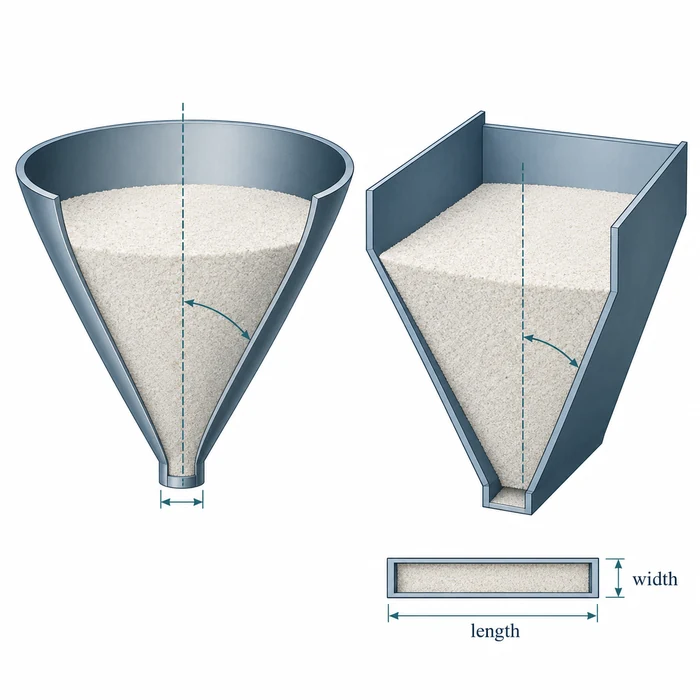
Conical and wedge hoppers require different design charts. The critical outlet dimension is a diameter for the cone and a slot width for the wedge.
A shear-test report provides a material flow function, friction angles, and bulk density measurements. The proposed hopper has a wall angle, an outlet dimension, and a withdrawal device. The engineering task is to establish whether that combination will support the intended discharge conditions.
Two questions govern the initial assessment: can the material move along the selected hopper walls, and is the opening large enough to prevent cohesive arching? This procedure follows both calculations through a worked example, then examines storage history and feeder operation before reaching a design decision.
1. Define the candidate and the operating case
Start with the equipment drawing and identify the hopper type, wall half-angle θ, outlet shape, clear dimensions, contact surface, and withdrawal device. Measure θ from vertical, as in Jenike’s charts. A smaller half-angle means a steeper wall. For example, a 20° half-angle from vertical corresponds to a 70° wall slope from horizontal. Record the angle convention wherever a value is reported.
For a conical hopper, the cohesive-arching dimension B is the circular outlet diameter. For a wedge hopper operating approximately in plane flow, B is the slot width. Jenike’s plane-flow approximation requires a slot length L greater than three times its width B (L > 3B). That geometric condition does not guarantee that material is withdrawn along the full slot.
Measure the effective clear opening after accounting for liners, gates, transitions, and parts projecting into the flow path. The nominal diameter or width may exceed the actual restriction at the feeder connection.
Define the material envelope: grade, representative batch variation, fines, moisture, temperature, handling history, maximum loaded standstill, and discharge duty. Separate continuous discharge from restart after storage. Each case may have its own strength and friction data.
Fill level helps establish the loading history and the stress range for testing, but the stress field in a hopper cannot be determined from liquid-like overburden pressure alone. Wall friction supports part of the load, while the converging section changes the stresses acting on the material. Record fill and withdrawal conditions alongside the test range.
1. Identify the hopper geometry and angle convention.
2. Measure the effective opening, including any liner, gate, transition, or intrusion.
3. Define continuous-flow and loaded-restart cases.
4. Agree the material conditions and stress range to be represented in testing.
2. Audit the laboratory outputs before calculating
Request the material flow function as paired values of major principal consolidation stress σ₁ and unconfined yield strength f꜀. These are derived shear-test quantities. The applied preshear normal load is not automatically σ₁, so instrument load settings alone are insufficient for this calculation.
Also obtain the effective angle of internal friction δ, the wall yield locus measured against the intended contact surface, and bulk density with its preparation and consolidation basis. Retain stress-dependent measurements rather than selecting a single convenient friction angle or density.
Wall friction deserves particular attention near the outlet, where normal stresses can be low. For a conventional curved wall yield locus, the wall-friction angle φ′ often increases as normal stress decreases. Use the angle corresponding to the relevant low wall-normal stress, commonly the governing condition for mass-flow design. Wall normal stress and major principal consolidation stress σ₁ are different quantities; choose the friction input using the appropriate wall-stress assessment.
Where bulk density changes with consolidation, request a density-versus-stress relationship. After locating the critical intersection, select a density representative of the critical outlet condition rather than substituting skeletal density or an unrelated loose-fill or tapped-density value.
ASTM D6128-22 covers testing with the Jenike shear tester, and ASTM D6773-22 covers testing with the Schulze ring shear tester. Specify the method edition, sample conditioning, test history, and stress range. Method selection is explained further in Jenike shear cell versus ring shear tester.
| Required output | What it contributes | Audit question |
|---|---|---|
| σ₁ and f꜀ pairs | Material strength curve | Does the measured range bracket the design crossing? |
| Effective internal friction δ | Chart family and hopper flow factor | Is its stress dependence represented? |
| Wall-friction data | Mass-flow boundary and flow-factor selection | Does the coupon represent the service surface and low-stress range? |
| Bulk density ρᵦ | Strength-to-outlet conversion | Is density representative of the critical outlet condition? |
| Time-consolidated strength | Loaded-restart assessment | Does the hold represent the intended standstill? |
PTI’s Flow Function / ffc Interpreter accepts measured σ₁ and f꜀ pairs, plots the material flow function, and calculates pointwise flowability coefficients. Use it to inspect the dataset before applying the geometry-specific wall-angle and outlet calculations.
3. Check wall-angle suitability and select the hopper flow factor
Select the mass-flow chart for the candidate geometry, measured effective internal friction, and governing wall-friction condition. Jenike’s Bulletin 123 presents conical-flow charts in Figures 45–49 and plane-flow charts in Figures 50–57. Read the limiting wall half-angle from vertical and compare it with the candidate θ.
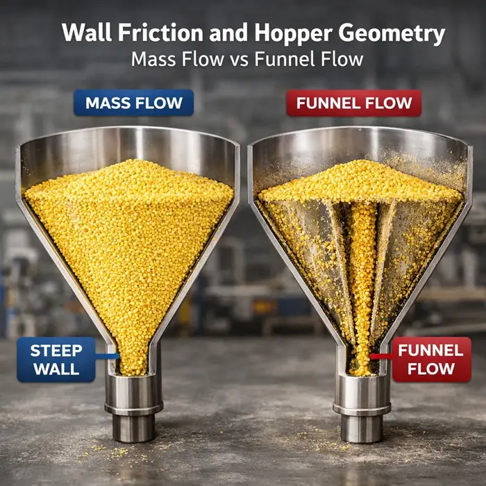
Mass flow requires powder to slide along the converging boundary while deforming internally. As explained in Wall friction and hopper geometry, increasing outlet size cannot independently correct a wall that is too shallow or too rough. Conversely, steeper walls do not eliminate cohesive strength at the opening.
For an actual mass-flow design, select a wall angle inside the theoretical limit with an appropriate allowance for material variation, surface condition, and fabrication. Mehos and Morgan recommend a 3° allowance for round or square outlets. Apply that guidance to the stated geometries rather than transferring it automatically to wedge hoppers. Record the selected chart, friction inputs, interpolation, limiting angle, and design allowance.
Read the hopper flow factor ff for the selected geometry, wall angle, wall friction, and effective internal friction. It describes the modeled hopper-material combination and differs from the material flowability coefficient ffc:
ffc = σ₁ / f꜀
The coefficient ffc describes the material at a particular consolidation state; ff belongs to the hopper calculation. A powder classified as easy flowing can still encounter discharge problems in unsuitable equipment. When the candidate wall angle or liner changes, revisit ff and the critical intersection rather than substituting an ffc classification for ff.
4. Locate the critical intersection
Plot unconfined yield strength f꜀ on the vertical axis against major principal consolidation stress σ₁ on the horizontal axis, using the same stress units. Draw the hopper flow-factor line through the origin with slope 1/ff:
f꜀ = σ₁ / ff
At its intersection with the measured material flow function, the stress available to overcome a cohesive obstruction equals the material’s unconfined yield strength. Read the critical unconfined yield strength f꜀,crit on the vertical axis and the corresponding consolidation stress σ₁,crit on the horizontal axis.
The outlet equation uses f꜀,crit, not σ₁,crit. Substituting the horizontal coordinate would inflate the calculated dimension by a factor of ff.
Keep the measured points visible and interpolate between them only where the observed curve shape justifies doing so. An apparent crossing outside the measured stress range needs further measurements or an explicitly supported extrapolation. If stress-dependent friction changes the selected ff, repeat the chart and intersection steps until the inputs are consistent.
An unusual concave-upward material flow function can intersect the hopper line more than once, as Jenike describes. Calculate the opening associated with each relevant intersection. The largest required dimension governs.
| Curve relationship | Interpretation | Next action |
|---|---|---|
| One clear crossing from above to below the hopper line as stress increases | A minimum-opening critical strength can be identified within the model | Calculate the outlet dimension and examine sensitivity |
| Material curve below the hopper line over the tested range | No crossing is demonstrated in that range | Establish whether the relevant low-stress region is covered |
| Material curve above the hopper line over the tested range | Gravity-flow adequacy is not demonstrated | Review geometry, surface, conditioning, and missing stress coverage |
| Multiple crossings from a concave-upward flow function | The intersection giving the largest required opening governs | Identify all relevant crossings and calculate the governing opening |
| Reverse-direction, near-tangent, or fit-dependent crossings with no clear governing intersection | A minimum-opening design point is unresolved | Obtain additional measurements and specialist interpretation |
For a complete idealized model, a material flow function entirely below the hopper line gives no minimum opening imposed by cohesive arching; a function entirely above the line indicates that the modeled gravity stresses cannot overcome the material’s strength. A finite laboratory dataset supports conclusions only within its tested stress range. Where the curve stays on one side of the line, establish whether the missing lower-stress or higher-stress region changes the design verdict.
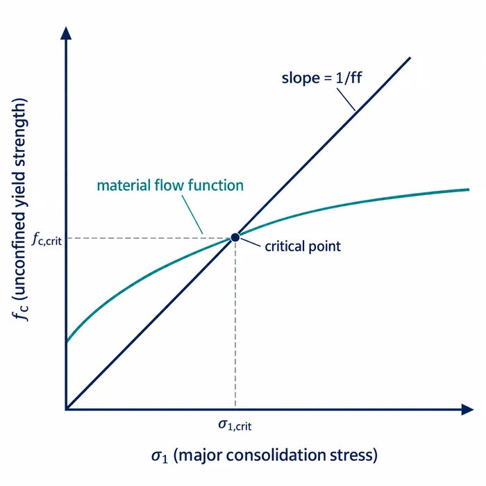
The intersection identifies critical unconfined yield strength on the vertical axis and critical consolidation stress on the horizontal axis. The outlet calculation uses the vertical coordinate.
5. Convert critical strength into the required opening
The critical yield strength determines the minimum opening against cohesive arching within the selected hopper model. Read the dimensionless outlet function H(θ) from Jenike’s Figure 43 for the appropriate opening geometry and wall half-angle. H is different from ff: the latter determines the intersection, while H converts critical strength into an outlet dimension.
Bcrit = H(θ) × f꜀,crit / (ρᵦ × g)
Here Bcrit is the critical circular diameter or slot width in meters; f꜀,crit is in pascals; ρᵦ is bulk density in kg/m³; and g is gravitational acceleration, approximately 9.81 m/s². Convert strengths given in kilopascals to pascals before calculating.
Use a bulk density representative of the material near the outlet under the critical consolidation condition. If density varies significantly with consolidation, select or interpolate ρᵦ using the density-versus-stress measurements at approximately σ₁,crit, and examine sensitivity to that selection. Skeletal density and an unexplained tapped-density result are unsuitable substitutes.
When bulk weight density γ is given directly in N/m³, gravity is already included (γ = ρᵦ × g), so the equation becomes Bcrit = H(θ) × f꜀,crit / γ. This distinction is important when reproducing calculations in pound-force and feet.
Compare Bcrit with the effective clear outlet dimension. Equality represents the theoretical critical boundary. Select an engineering allowance that accounts for property variation, interpolation uncertainty, fabrication tolerance, and the operating envelope. Preserve both the calculated dimension and the final selected opening in the design record.
A liner may improve wall friction while reducing the clear opening; a partially open gate may create a smaller restriction than the hopper outlet. Recheck the effective dimension whenever the equipment arrangement changes.
6. Worked example: recalculating Jenike’s cone and slot
Jenike’s Example 4(a), on pages 150–153 of Storage and Flow of Solids, compares a conical hopper with a plane-flow solution for an unnamed material characterized using a time-consolidated flow function. The original example includes a chart-based flow-factor selection and an iteration for plane flow, rather than starting directly from an outlet size.
Jenike first assumes ff ≈ 1.3 and draws the corresponding line on the flow-function construction in Figure 96. The intersection gives a major principal consolidation force of approximately 4.7 lbf. Using the effective internal friction of 50° and wall friction of about 24°, Figure 47 gives a limiting conical wall half-angle of 17° and ff = 1.28, close enough to the initial estimate for this solution. The critical unconfined yield force is 3.65 lbf.
For plane flow, the initial chart selection yields a 28° wall half-angle and ff = 1.20. Jenike repeats the construction, obtaining effective internal friction of 52°, wall friction of 26°, and a limiting half-angle of 25°. Interpolation between Figures 52 and 53 gives ff = 1.17 and a critical unconfined yield force of 3.3 lbf. The final inputs from the published example appear below.
| Input | Conical solution | Plane-flow solution |
|---|---|---|
| Wall half-angle θ from vertical | 17° | 25° |
| Hopper flow factor ff | 1.28 | 1.17 |
| Critical yield force F | 3.65 lbf | 3.3 lbf |
| Outlet function H | 2.27 | 1.13 |
| Shear-cell area A | 1/13 ft² | 1/13 ft² |
| Bulk weight density γ | 50 lbf/ft³ | 50 lbf/ft³ |
Jenike expresses critical strength as yield force F divided by shear-cell area A. With A = 1/13 ft², the conical strength is 3.65 × 13 = 47.45 lbf/ft², and the plane-flow strength is 3.3 × 13 = 42.9 lbf/ft².
The original example uses a constant bulk weight density γ of 50 lbf/ft³. Because this quantity already includes gravity, the corresponding outlet equation is:
Bcrit = F × H / (A × γ)
Bcrit,cone = 13 × 3.65 × 2.27 / 50 = 2.15423 ft = 0.656609 m
Bcrit,slot = 13 × 3.3 × 1.13 / 50 = 0.96954 ft = 0.295516 m
Using 1 ft = 0.3048 m, the theoretical critical dimensions are a 657 mm conical outlet diameter and a 296 mm plane-flow slot width. The slot-length condition L > 3B gives L > 2.91 ft, so a 3 ft slot meets the geometric approximation.
A separate SI check gives f꜀,crit = 2,271.9 Pa for the cone and 2,054.1 Pa for plane flow, using 1 lbf/ft² ≈ 47.8803 Pa. Multiplying by the final flow factors gives σ₁,crit ≈ 2,908.1 Pa and 2,403.3 Pa, respectively. Converting γ = 50 lbf/ft³ gives approximately 7,854.4 N/m³. These values reproduce the calculated outlet lengths.
The smaller slot width does not indicate a smaller outlet area, and it cannot replace the diameter of a circular opening. Each geometry has its own flow factor, outlet function, and governing material strength.
Two assumptions matter when transferring this example to equipment design. Jenike calculates at the theoretical limiting wall angles of 17° and 25°, whereas a working mass-flow design includes an appropriate angular allowance and then revisits ff, the intersection, H, and Bcrit. The published example also uses one constant bulk weight density. For a material with significant stress-dependent density, use a representative density for the critical outlet condition as discussed in Section 5. The calculated dimensions are theoretical results, not final equipment specifications.
7. Check storage, wall condition, and withdrawal
The wall-angle and cohesive-arching calculations provide only part of the discharge assessment. Test conditions and equipment operation must represent the intended service case.
When material remains under load before restart, repeat the flow-function intersection using the relevant time-consolidated strength data. Consolidation during storage can increase strength and the required opening. Select a hold duration and stress history representative of the maximum intended standstill rather than relying exclusively on fresh-flow results.
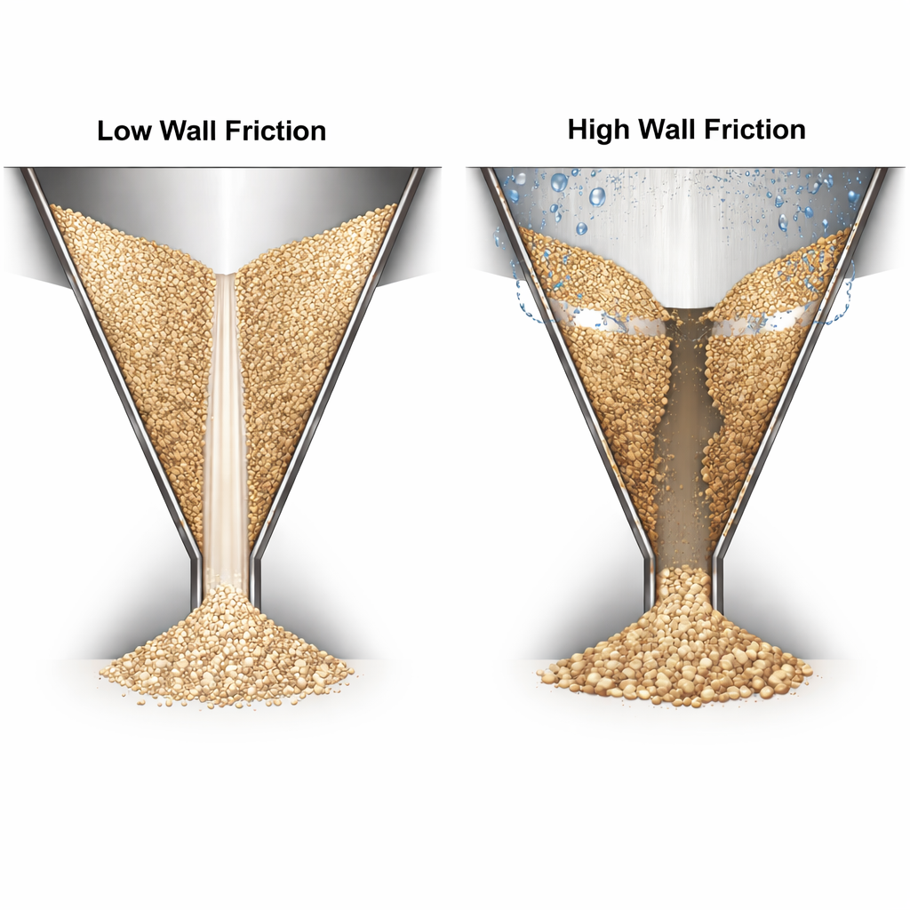
The contact surface must also represent service conditions. A clean laboratory coupon may differ from a worn liner or a wall coated with product. Wall friction drift in hoppers explains how these changes can alter discharge behavior. Obtain representative wall-friction measurements where the existing coupon no longer reflects the operating surface.
An unusual concave-upward wall yield locus can shift the governing stress condition above the outlet. Jenike’s method addresses that case by checking the critical dimension at several hopper elevations. This is distinct from the multiple-intersection behavior of a concave-upward material flow function described in Section 4.
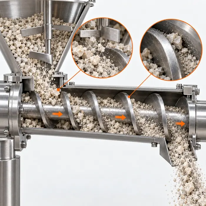
Inspect the withdrawal arrangement below the opening. A long slot above a screw may experience localized extraction even when the nominal width meets the arching calculation. Confirm that material is drawn along the required active length and that the feeder can accept the incoming discharge without obstructing or overcompacting the bed. Where the interface imposes additional loads, evaluate those boundary conditions separately.
Ratholing is a different failure mechanism. If funnel flow is possible or intentional, assess whether a stable channel can remain within the surrounding material using the appropriate consolidation state and rathole method. The cohesive-arching calculation does not determine whether the stagnant bed will collapse. See Storage and discharge for the broader handling context.
Finally, check discharge rate and coarse-particle passage. Fine-powder flow may be restricted by gas movement and permeability, while coarse particles may interlock mechanically at narrow openings. Determine these constraints using suitable tests or calculations before finalizing the opening.
8. Record a decision that leads to the next action
Close the review with separate verdicts for wall-angle suitability, cohesive arching, loaded restart, and withdrawal. A satisfactory theoretical outlet dimension cannot compensate for unsuitable walls or a feeder that extracts material unevenly. Record the material conditions and equipment geometry evaluated with each result.
| Outcome | Record | Next action |
|---|---|---|
| Candidate meets the evaluated criteria | Chart basis, crossing, critical dimension, selected allowance, represented operating cases | Complete rate and interface verification and define commissioning acceptance |
| Candidate misses a criterion | Controlling wall-angle or outlet shortfall | Revise geometry, surface, opening, or material condition and repeat the affected checks |
| Evidence is insufficient | Missing stress coverage, unresolved crossing, untested hold, surface mismatch, or interface load | Request the specific missing measurement or application analysis |
Bring the equipment drawing, shear-test report, wall-friction measurements, selected charts, critical intersection, density basis, calculated outlet dimension, and outstanding operating checks into one record. Retain the theoretical and selected equipment dimensions separately. If a required input is missing, identify the measurement or engineering analysis needed before assigning a design acceptance result.
Hopper Design-Check Workbook: Shear Data, Wall Angle, and Outlet Size
The companion design-check workbook is intended to capture the test-request checklist, chart selection, critical intersection, outlet calculation, and decision record. Confirm that its inputs, figures, and calculations match the reviewed operating case before using it to support equipment selection.
Technical Basis / Sources
– Jenike, Andrew W. Storage and Flow of Solids. Bulletin No. 123, Utah Engineering Experiment Station, University of Utah, November 1964. Sixth printing, revised March 1970.
– Schulze, Dietmar. Powders and Bulk Solids: Behavior, Characterization, Storage and Flow. 2nd edition. Springer, 2021.
– Mehos, Greg, and Dave Morgan. “Hopper Design Principles.” Chemical Engineering, January 2016.
– ASTM International. ASTM D6128-22: Standard Test Method for Shear Testing of Bulk Solids Using the Jenike Shear Tester.
– ASTM International. ASTM D6773-22: Standard Test Method for Bulk Solids Using Schulze Ring Shear Tester.