Table of contents
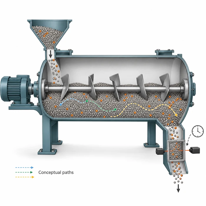
Two continuous powder lines can deliver the same throughput and have the same average residence time, yet respond differently when an ingredient feed changes. One may deliver a compact concentration excursion. Another may show an early response followed by a small contribution that persists much longer. The average conceals the timing that matters to the next operation.
Residence time distribution, or RTD, describes how transit times are distributed among portions of material passing between defined process boundaries. This article explains how to measure that distribution and turn it into a useful engineering decision. The experimental example comes from pharmaceutical continuous blending; applications elsewhere require measurements representative of the material and equipment involved.
The average conceals who leaves early and who stays late
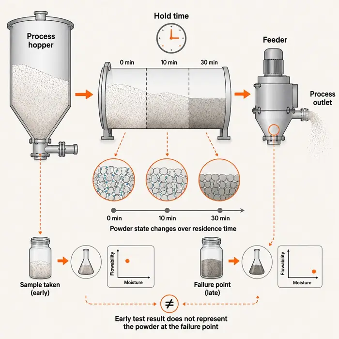
Powder condition can change while material waits between operations, as discussed in Powder Residence Time Can Make the Test Result Miss the Failure. RTD addresses a complementary question: how widely do transit times differ within the moving stream? That distinction matters when matching an upstream event to downstream samples or deciding how long a transition affects collected product.
Consider a calculated example with an instantaneous tracer pulse and complete recovery. In distribution A, half the tracer exits at 50 seconds and half at 70 seconds. In distribution B, 90% exits at 40 seconds and 10% at 240 seconds. These idealized exit fractions demonstrate the distinction without introducing assumptions about a fitted curve.
| Calculated characteristic | Distribution A | Distribution B |
|---|---|---|
| Tracer exit fractions | 50% at 50 s; 50% at 70 s | 90% at 40 s; 10% at 240 s |
| Mean residence time | 60 s | 60 s |
| Variance | 100 s² | 3,600 s² |
| Tracer exited by 70 s | 100% | 90% |
The mean is the fraction-weighted exit time: distribution B gives 0.9 × 40 + 0.1 × 240 = 60 seconds. Its late fraction compensates for the earlier exit of most material. A collection rule based on the mean would therefore describe neither the first arrival nor the final contribution. The calculation demonstrates different timing, without assigning either distribution a product-quality outcome.
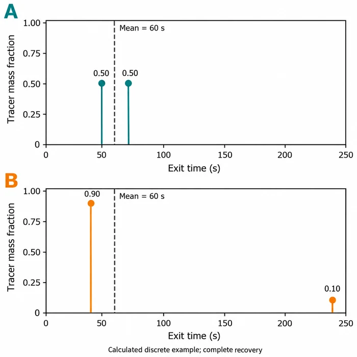
Calculated example with complete recovery: both means are 60 s, while variances are 100 s² and 3,600 s². Stems represent discrete exit fractions.
Define the process boundary before interpreting the curve
An RTD belongs to an inlet, an outlet, a material, and an operating condition. A measurement across a blender differs from one spanning its feeder, connecting chute, blender, and receiving equipment. Record those boundaries first. Otherwise, an apparent change in blender behavior may actually reflect an altered transfer path or measurement location.
Working hold-up divided by steady mass throughput gives an inventory turnover estimate. For example, 2 kg ÷ 120 kg/h = 1/60 h; multiplying by 3,600 s/h gives 60 seconds for this idealized estimate. Relating that estimate to a tracer mean requires representative hold-up and a steady material balance. Nominal vessel capacity can include space or retained material that does not participate in the measured flow.
ICH Q13 describes RTD in pharmaceutical continuous manufacturing as specific to the process, composition, material properties, equipment design, and configuration [1]. Physically, different transport paths can produce early passage, while recirculation or exchange with slowly moving regions can prolong exit. These are mechanisms to investigate, rather than unique diagnoses obtainable from curve shape.
Relate characterization to the powder operating window: a test at one rate and powder condition does not establish the response after a change in fill, formulation, moisture, or configuration. When comparing settings, record the conditions that could change particle movement and repeat the measurement where the resulting control decision will be used.
Measure the input as carefully as the outlet
A pulse test introduces a brief, measurable quantity of tracked material and follows its outlet response. A composition step changes an inlet constituent from one level to another and follows the transition. Q13 recognizes composition step testing as an alternative to an external tracer [1]. Choose the approach around detectability and whether the imposed change preserves the process behavior being characterized.
Tracer fidelity is central. Q13 recommends highly similar flow properties to the replaced constituent, inertness toward other components, and no alteration of material interactions with equipment surfaces [1]. A readily detected tracer that segregates, adheres, or agglomerates differently may describe its own path more strongly than the constituent of interest.
A finite inlet pulse already has a duration. Feeder delivery and injection hardware can broaden it before the material reaches the test boundary. Record the actual input timing where feasible and distinguish input width from downstream spreading. An outlet curve cannot automatically be treated as the equipment’s response to an instantaneous pulse.
- Define inlet and outlet boundaries, operating state, tracked constituent, and the decision the test must support.
- Establish baseline behavior, analytical calibration, timestamp alignment, and the actual inlet change.
- Collect time-resolved outlet measurements through breakthrough, the main response, and the measurable tail.
- Check recovery and measurement limitations before comparing metrics or fitting a model.
- Repeat relevant conditions to separate reproducible transport behavior from run-to-run and measurement variation.
Physical sampling and inline sensing solve different parts of the problem. Full-stream increments can support representative composition measurements, but combining them into one composite destroys the time history needed for RTD. Apply representative powder sampling principles while retaining each increment’s collection interval. For a local optical probe, assess whether its observed material represents the stream crossing the outlet.
Turn concentration measurements into a distribution
For an effectively instantaneous pulse, constant outlet mass flow, and a representative concentration measurement, subtract the baseline concentration and normalize the response by its area. The result, E(t), is an exit-time density with units of inverse time. Its cumulative integral, F(t), is the fraction of recovered tracer that has exited by time t.
E(t) = [C(t) − C₀] /
F(t) = ∫₀^t E(u) du
Here, C(t) is outlet tracer concentration, C₀ is the baseline, and u is an integration variable. If flow varies, concentration area alone does not represent tracer mass: recovery accounting must include outlet mass flow. A large disturbance can also change the transport itself, requiring a treatment beyond a single stationary RTD.
Keep absolute recovery separate from normalization. A curve normalized to unit area can look complete even when the observation window missed retained tracer. A truncated tail understates late contributions and can bias the mean and variance. Report the observation duration, reporting limit, baseline treatment, and recovered quantity alongside the normalized curve.
For a stable, linear transport response, a normalized rising step can represent F(t). Its derivative then gives E(t), although differentiation amplifies measurement noise. Inspect the cumulative response before differentiating it. Sampling intervals, instrument averaging, and sensor response should resolve the timing relevant to the intended decision.
What the pharmaceutical blending example demonstrates
An FDA poster by M. Krull, N. Pavurala, and T. F. O’Connor examined acetaminophen, lactose monohydrate, and microcrystalline cellulose in a continuous tubular blender [2]. The researchers developed predictive RTD models at 5% and 30% acetaminophen loading, with total flow rates of 10–25 kg/h.
The setup used an NIR probe below the blender outlet and collected spectra approximately once per second. NIR calibration-model accuracy was checked against offline HPLC measurements of blend samples. This distinction is useful: the rapid concentration estimate came from a calibrated spectral model, with a separate analytical method used to assess its accuracy.
The poster reported stronger external predictive performance for the 5% loading than for the 30% loading. Greater NIR variability and less stable normalization baselines accompanied the weaker performance at the higher loading [2]. Before attributing a changed RTD to powder transport, therefore, examine whether the concentration measurement and baseline remain dependable.
The researchers used a tanks-in-series model, a mathematical representation of successive mixed volumes. Such a model can compactly describe a response without establishing that the blender contains equivalent physical compartments. For practical use, evaluate predictions at independent conditions and against the timing features needed by the control strategy.
Read shape in relation to the production decision
Distribution width describes spreading in exit time. Under a linear, time-invariant transport approximation, the outlet concentration history equals the inlet concentration history convolved with the normalized RTD, E(t). This convolution relationship is why spreading can reduce the peak of some short inlet concentration disturbances while extending their downstream duration. It does not remove the added material. Sustained feed errors and changes that alter process behavior need separate evaluation.
This makes a refill event a useful diagnostic starting point. Loss in Weight Feeder Drift After Refill explains how changing powder state can create an inlet disturbance. Measure that disturbance and compare it with the downstream response. A smaller outlet peak may reflect temporal redistribution even while the transition lasts longer.
| Measured feature | Engineering question | Next discriminating check |
|---|---|---|
| Early breakthrough | Does part of the tracked material arrive before collection logic expects? | Check inlet timing, boundary locations, and possible preferential paths. |
| Wide main response | How far does an inlet disturbance spread in time? | Compare measured inlet and outlet histories at the relevant operating state. |
| Persistent tail | How long does a measurable contribution remain? | Extend observation and inspect slowly exchanging regions or deposition. |
| Different responses between repeats | Did transport change, or did measurement change? | Check operating records, baseline, calibration, sampling, and recovery. |
RTD also provides a time framework for transformations. A dryer or granulator must expose material to the required processing conditions, but transit time alone does not establish moisture, granule structure, or thermal history. In blending, the mixing and blending guide provides the complementary framework for composition uniformity. Pair transport measurements with the product attribute the operation must deliver.
For grade transitions, a tail supports an estimate of continued contribution from the tracked material. It does not establish validated cleanliness. Adhered residues or material released during a later disturbance may escape the test’s observation. Use RTD to inform transition planning, and use the applicable residue and cleaning verification methods for cleanliness decisions.
Specify the decision before choosing the model
Select metrics around the intended action: early exit for first-arrival timing, mean and variance for transport comparison, and cumulative exit fractions for transition tracking. Define percentile notation explicitly, such as t₉₅ for the time by which 95% of recovered tracer has exited. No percentile is a universal product-collection threshold.
Q13 connects RTD with sampling, traceability, and diversion, while also recommending consideration of disturbance severity and measurement and diversion locations [1]. A usable diversion strategy must account for detection delay, downstream travel, actuator response, and uncertainty. Its start and stop criteria need a demonstrated relationship to the product acceptance requirement.
The FDA poster describes its RTD models as medium-impact models because of their potential use in feedforward control [2]. Q13 recommends development, validation, and lifecycle documentation proportionate to model type and impact [1]. The practical implication is to test the prediction used by the decision, including independent runs and relevant operating changes.
Start with one consequential event on the line: a refill, recipe transition, or planned composition change. Define its inlet history and downstream acceptance requirement, then measure the response across the actual collection boundary. Use the resulting breakthrough, spread, and tail to decide whether sampling timing, collection logic, or physical transport needs the next investigation.
Technical Basis / Sources
- U.S. Food and Drug Administration, Center for Drug Evaluation and Research and Center for Biologics Evaluation and Research. (2023, March). Q13 Continuous Manufacturing of Drug Substances and Drug Products: Guidance for Industry. ICH.
- Krull, M.; Pavurala, N.; O’Connor, T. F. Predictive Residence Time Distribution Models for Continuous Powder Blending. Poster. Office of Pharmaceutical Quality, Center for Drug Evaluation and Research, U.S. Food and Drug Administration.