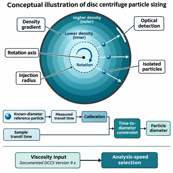

Identical particles can produce different settling velocities when concentration changes. Conceptual illustration, not experimental data.
A suspension interface settles more slowly than the isolated-particle reference. Feeding that interface velocity into a Stokes sizing equation then reports a smaller diameter. How much smaller, and does the difference justify a correction? The calculation is straightforward; deciding whether it represents the suspension requires a separate check.
Why a slower interface looks like a smaller particle
Stokes sizing converts terminal velocity into an equivalent spherical diameter. A concentrated interface instead follows collective suspension motion: particles displace liquid upward, and hydrodynamic interactions change their descent. PTI’s distinction between settling regimes explains why these observables require different interpretations.
Let d0 be the isolated-sphere diameter, u0 its terminal velocity, and uh the suspension-interface velocity. With viscosity η, density contrast Δρ and gravity g fixed, the Stokes inversion gives:
dapp = sqrt(18ηu_h/(Δρg)); dapp/d0 = sqrt(uh/u0)
ISO 13317-1:2024, superseding ISO 13317-1:2001, defines these Stokes-diameter principles for gravitational sedimentation sizing; its scope excludes sedimentation at high particle concentrations, including zone settling, so the worked example below falls outside it. Velocity in m/s, viscosity in Pa·s, density contrast in kg/m³ and gravity in m/s² give diameter in metres; the ratio is dimensionless. Inserting interface velocity into this isolated-particle inversion is a diagnostic calculation, not a validated sizing procedure.
A conditional 10% solids example
Consider the same uniform, nonaggregating spherical population in the same liquid, temperature and gravitational field, with preparation and observation history defined. Concentration changes; diameter and liquid properties stay fixed. Richardson’s author commentary reports n approximately 4.65 for particle Reynolds numbers below about 0.2, with negligible wall effects.
uh/u0 = (1 − φ)^n
Here φ is solids volume fraction, not mass fraction.
With φ = 0.10 and n = 4.65, the model gives uh/u0 ≈ 0.6127 and dapp/d0 ≈ 0.7827, an apparent diameter about 21.7% below d0.
Combining the two relationships gives a single ratio between apparent and reference diameter, and inverting it gives a conditional correction:
dapp/d0 = sqrt((1 − φ)^n); d0 = dapp/sqrt((1 − φ)^n)
This inverse is a conditional model inversion, valid only where φ and n are known and the model’s assumptions hold, not a universally valid or experimentally validated particle-size correction.
| Solids volume fraction, φ | Underestimation, n = 4.65 | Underestimation, n = 5.1 (illustrative) |
|---|---|---|
| 1% | 2.3% | 2.5% |
| 5% | 11.2% | 12.3% |
| 10% | 21.7% | 23.6% |
| 20% | 40.5% | 43.4% |
The n = 5.1 column illustrates exponent sensitivity, not an interchangeable universal exponent; both columns are model predictions, not measurements. Underestimation varies nonlinearly with solids volume fraction; concentration uncertainty must therefore be propagated at the concentration being assessed.
Decide whether correction is defensible
Richardson–Zaki can be linearised: ln(uh) = ln(u0) + n ln(1 − φ). A velocity series measured across controlled concentrations gives a fitted exponent from the slope and an isolated-particle velocity from the zero-concentration intercept, convertible to a Stokes-equivalent diameter under the same assumptions. That fitted diameter is model-derived, not an independently validated particle diameter: the fit alone cannot confirm unchanged particle association, model validity, or freedom from confinement and other systematic effects.
When measured settling differs from the prediction, work through a defined sequence rather than assuming hindrance alone explains it:
- Check the original height-time records: fitting windows, concentration units, temperature, vessel geometry, and measurement uncertainty.
- Measure initial settling velocity at several controlled solids volume fractions, excluding compression and consolidation intervals.
- Plot ln(uh) against ln(1 − φ); assess linearity and compare the fitted exponent with the applicable prediction for the measured particle Reynolds number.
- Compare the zero-concentration intercept with an independent dilute-settling reference, accounting for wall effects where relevant.
- Verify particle-state stability independently, particularly whether dilution changes aggregation or dispersion.
Exponent agreement alone does not prove hindrance is the only mechanism; aggregation, polydispersity, and confinement can produce similar trends. Preserve liquid composition, temperature, and preparation history when comparing concentrations, since dilution can change the particles measured and their hydrodynamic interactions, as PTI’s guidance on preserving the tested dispersion state explains. If the assumptions fail, or the diameter cannot be validated, report interface velocity, concentration, and conditions as model inputs rather than a particle-size result, and use the slurry troubleshooting route to select the next measurement.
Technical Basis / Sources
- Richardson, J. F. (1979, February 12). Citation Classic commentary on Richardson and Zaki (1954), Sedimentation and fluidisation, Part 1. Commentary dated June 30, 1978, p. 243.
- International Organization for Standardization. (2024). ISO 13317-1:2024, Determination of particle size distribution by gravitational liquid sedimentation methods — Part 1: General principles, requirements and guidance. Second edition, April 2024.
- Richardson, J. F., and Zaki, W. N. (1954). Sedimentation and fluidisation: Part I. Transactions of the Institution of Chemical Engineers, 32, 35–53. Reprinted in Chemical Engineering Research and Design, 75, S82–S100 (1997). https://doi.org/10.1016/S0263-8762(97)80006-8.